In this article we provide a brief overview of our work Multi-View Networks For Multi-Channel Audio Classification. In this work we propose a neural network architecture that performs audio classification/event detection given recordings from multiple devices.
Motivation
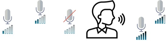
Suppose we’re in a meeting room and there’s a speaker talking. Now we would like to perform some audio sensing task, identifying whether the speaker is talking or not at a given time. Each of us are likely to have a couple of recording devices by our hand, such as our cellphones and laptops; however, not all of them are recording all time. What’s more, the recording quality of each device might be different: some device will provide clean recordings, while others yield poor quality recordings due to the distance to the speaker or defects of the devices themselves. It would therefore be nice to have a system that can perform audio classification/detection from any number of devices and the performance will not degrade because of the channels with poor recording quality.
Problem Description
Not all devices are recording at all time steps, and the quality of the signal recorded is different between devices.
In recent years, deep neural networks have been explored in one-channel or two-channel audio classification(here we assume that the signal from each channel corresponds to the recording from one device), and the models have been extended to multi-channel tasks as well. However, previous deep learning models only can only be applied for a fixed number of channels. First, the number of devices with which the models are deployed must be the same as the number of devices of the recordings in the training set. Second, these models cannot deal with the case where number of devices may varies from time to time. We propose the Multi-View Network that can handle the two issues above.
Multi-View Networks
Multi-View Networks(MVNs) are variants of Recurrent Neural Networks(RNNs), which are a common starting point for classifying ore predicting sequences(if you’re not familiar with RNNs, you may refer to this awesome post). Recall that an RNN may take sequences of arbitrary length since it unrolls across the time dimension. In other words, an RNN can be trained on sequences of length \(k\) and be tested on sequences of length \(k'\) where \(k \neq k'\).
Let’s return to the multiple recording classification task. We want a model that can handle input sequences with not only variable length but also varying number of channels. Hence, we need a model that unrolls across both the time and the channel dimension, and this is how we design the Multi-View Networks.
MVN Architecture
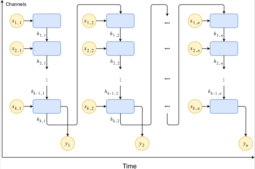
At each time frame, the model observes information across all channels before making a prediction. It passes the state of the last channel of the current time frame into next frame.
The diagram above illustrates how MVNs unroll across both time and channel dimensions. For each time frame, the model unrolls the input channel by channel. When it reaches the last channel, it passes the hidden state into the first channel of the next time frame and meanwhile predicts whether the current frame contains speech or not. By unrolling first across channel and then across time, the MVN by essence is a 2D RNN. The following equations represent the recurrence relation in MVN:
\[\begin{split} \mathbf{h}_{k, t} &= \begin{cases} \sigma(\mathbf{W}_h \mathbf{x}_{k,t} + \mathbf{U}_h \mathbf{h}_{k,t-1}) & , k = 1 \\ \sigma(\mathbf{W}_h \mathbf{x}_{k,t} + \mathbf{U}_h \mathbf{h}_{k-1,t}) & , 1 < k \leq K \end{cases} \end{split}\] \[\mathbf{y}_{t} = \sigma(\mathbf{W}_x \mathbf{h}_{K,t}) \notag\]where K is the number of channels, \(\mathbf{h}_{k, t}\) is the hidden state for the \(k\)-th channel at time \(t\), \(\mathbf{y}_t\) is the predicted label at time \(t\), and \(\sigma\) is the sigmoid function. The recurrence above allows the model to aggregate information from all channels at each time step.
Pipeline
Audio Classification with MVN
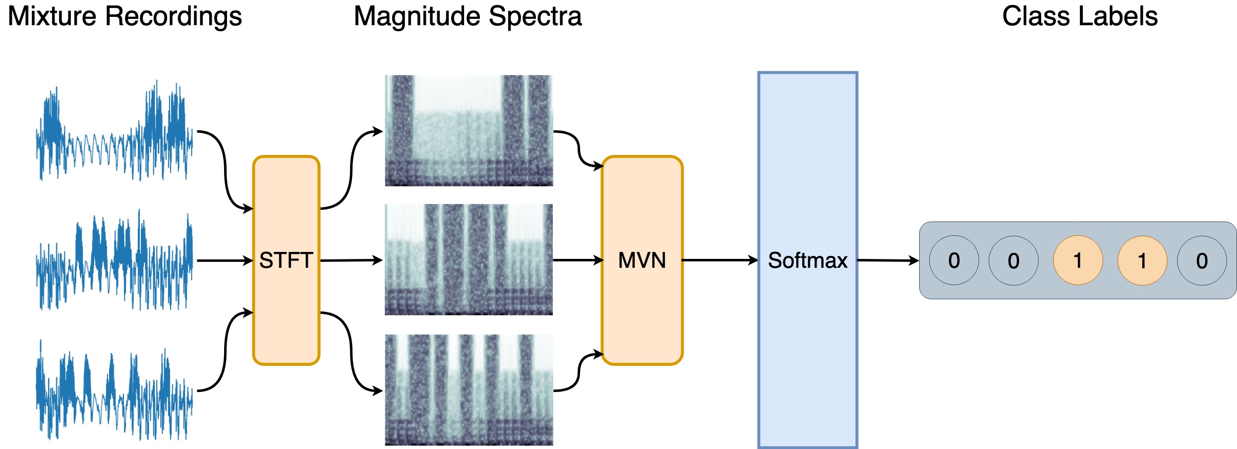
The diagram above illustrates the pipeline of audio classification/event detection with MVN. The pipeline can be summarized as following:
- Take the magnitude spectra of each channel using Short-Time Fourier Transform(STFT)
- Pass the magnitude spectra of all channels into MVN
- For each STFT frame, predict whether it’s background noise or event of interest
Notice that we did not discuss how to handle the delay between microphones with spatial difference. We assume that the delay is relatively small compared to the STFT window size(we use a window size of 1024 samples and a hop size of 512 in the experiments), so the small temporal difference may be ignored and therefore the discussion of alignment is not included in this work.
Conclusion
We list a few properties of the MVN architecture below:
- The performance is stable when the recording quality is different across devices. Compared to regular RNN models, MVN is less affected by channels with poor signal quality and is more effective at collecting information from few clean channels among many noisy channels.
- The performance is largely invariant to the order of the channels/devices. For MVN, it doesn’t matter which channels it sees first and which ones it sees later.
- The model can be deployed in settings with arbitrary number of devices.
If you’re interested in the experimental setups and results, please refer to the paper for a more detailed description. You may also check out our poster, which was presented at ICASSP 2019. The source code for MVN will be released within a few months.